Fire Experiment

Define and Run Simple Experiment

To run a NetLogo model simulation we have to create an experiment object with nl_experiment function. Experiment definition includes a NetLogo model file, declares how to run the model, defines parameter values and what outputs are expected from simulation runs.

For example:

experiment <- nl_experiment(
  model_file = "models/Sample Models/Earth Science/Fire.nlogo", 
  param_values = list(density = c(57, 59, 61)),
  while_condition = "any? turtles",
  random_seed = 1,
  export_view = TRUE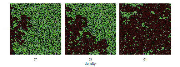
)

result <- nl_run(experiment)     

Find paths to the exported view image files in result$export or just display them by calling nl_show_views_grid function:

library(ggplot2)
nl_show_views_grid(result, x_param = "density")

Temporal Measures

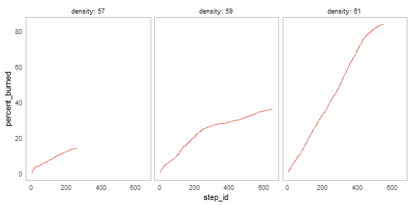
Temporal measures quantify temporal behavior of agent based model. Example below shows how to measure percent of burned trees on each simulation step:

\[ percent_{burned}(t) = \frac{trees_{burned}(t)}{trees_{initial}} \times 100 \]

To define a temporal measure use step_measures element. Measures have to be accurate NetLogo reporters.

experiment <- nl_experiment( 
  model_file = "models/Sample Models/Earth Science/Fire.nlogo", 
  while_condition = "any? turtles",
  param_values = list(density = c(57, 59, 61)),
  random_seed = 1,
  step_measures = measures(
    percent_burned = "(burned-trees / initial-trees) * 100",
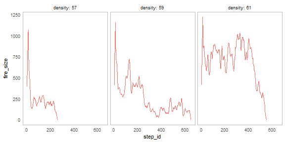
    fire_size = "count turtles"
  )
)

result <- nl_run(experiment)

To get the observations from the result object use nl_get_step_result:

dat <- nl_get_step_result(result)

head(dat)
#>   density param_set_id percent_burned fire_size step_id run_id
#> 1      57            1      0.4030340       395       1      1
#> 2      57            1      0.6437348       481       2      1
#> 3      57            1      0.8788379       565       3      1
#> 4      57            1      1.0859526       639       4      1
#> 5      57            1      1.3070615       718       5      1
#> 6      57            1      1.5113773       791       6      1

nl_show_step(result, y = "percent_burned", x_param = "density")

nl_show_step(result, y = "fire_size", x_param = "density")

Observations per each simulation run

Stochastic models are usually run several times repeteadly for each parameter set and measured at the end of each run.

In this example we observe percent of burned trees and fire progress for different density parameter. The model will run repetedly 30 times for every parameter value.

experiment <- nl_experiment(
  model_file = "models/Sample Models/Earth Science/Fire.nlogo", 
  while_condition = "any? turtles",
  run_measures = measures(
    percent_burned = "(burned-trees / initial-trees) * 100",
    progress = "max [pxcor] of patches with [pcolor > 0 and pcolor < 55]"
  ),
  repetitions = 30,
  param_values = list(
    density = seq(from = 55, to = 62, by = 1)
  )
)

When running experiments with several repetitions we can save some time with parallel option.

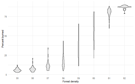
result <- nl_run(experiment, parallel = TRUE)  

dat <- nl_get_run_result(result)

One way to show the percent burned as a function of density is to use violin plot:

library(ggplot2)
ggplot(dat, mapping = aes(x = factor(density), y = percent_burned) ) + 
  geom_violin(fill = "gray90") +
  labs(x = "Forest density", y = "Percent burned") + 
  theme_minimal()

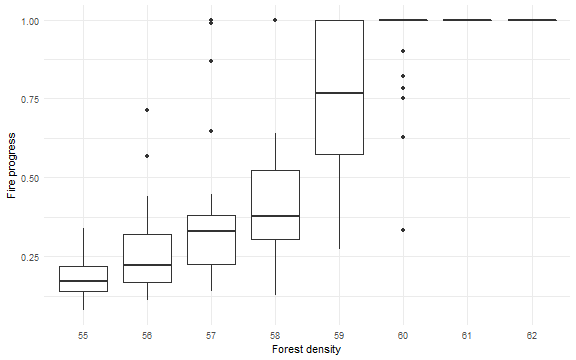
Fire advances from left to right. It is interesting to observe final fire position (left border = 0 and right = 1) as a function of density.

ggplot(dat, mapping = aes(x = factor(density), y = progress/250 + 0.5) ) + 
  geom_boxplot()  +
  #geom_jitter(position = position_jitter(width = .1), alpha = 0.3)  +
  labs(x = "Forest density", y = "Fire progress") +
  theme_minimal()

Aggregation Over Time

Sometimes a model does not have enough information at the end of simulation and can be measured only by aggregating some temporal measures over time.

One way to get aggregated data (e.g. maximum, mean or variance) is to report temporal measure and apply aggregation at the end of experiment run. But in case of long simulations it would require a lot of memory and aggregating measure at the and of each simulation run is more efficent.

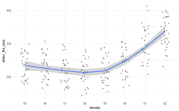
Use eval_criteria argument to define the aggreation of temporal measures. The following example define median and standard deviation of fire size (defined as number of trees with active fire in time \(t\)):

experiment <- nl_experiment( 
  model_file = "models/Sample Models/Earth Science/Fire.nlogo", 
  while_condition = "any? turtles",
  param_values = list(
    density = seq(from = 55, to = 62, by = 1)
  ),
  step_measures = measures(                                
    fire_size = "count turtles"                 # temporal measure
  ),
  eval_criteria = criteria (
    median_fire_size = median(step$fire_size),  # aggregate over iterations
    stdev_fire_size = sd(step$fire_size)
  ),
  repetitions = 30,                             # run simulation several times
  random_seed = 1:30                            # random seeds for repetitions
)

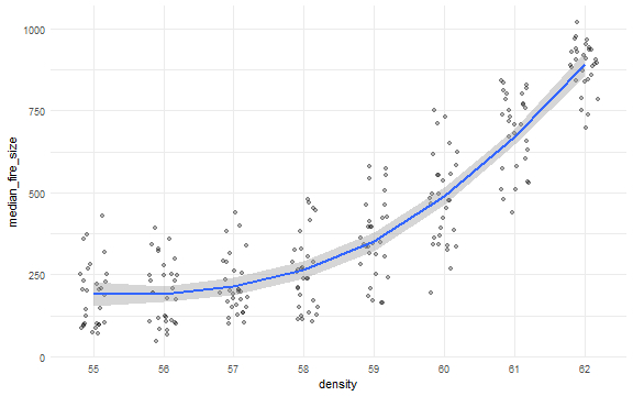
result <- nl_run(experiment, parallel = TRUE) 

dat <- nl_get_result(result, type = "criteria")
dat$density <- factor(dat$density)

ggplot(dat, aes(x = density, y = median_fire_size)) +
  geom_jitter(position = position_jitter(width = 0.2), alpha = 0.3) +
  stat_smooth(aes(group = 1), method = "loess") +
  theme_minimal()

dat <- nl_get_result(result, type = "criteria")
dat$density <- factor(dat$density)

ggplot(dat, aes(x = density, y = stdev_fire_size)) +
  geom_jitter(position = position_jitter(width = 0.2), alpha = 0.3) +
  stat_smooth(aes(group = 1), method = "loess") +
  theme_minimal()

Related

Segregation example demonstrates how to obtain data from individual NetLogo agents.

Network example demonstrates how to collect values from turtles and their links to recreate network as igraph object

Traffic example demonstrates how to collect values from turtles per each time step.

DLA example demonstrates how to read NetLogo patches.

Ants example demonstrates simple parameter sets definition and mapping.

Get rmarkdown source of this page.