This example is using NetLogo Flocking model (Wilensky, 1998) to demonstrate random search for optimal parameter values.

Like in the LHS example the Latin hypercube sampling method is used but instead of categorical criteria the simulations are evaluated with single best-fit criterion defined in Best-fit example.

library(tgp)

experiment <- nl_experiment( 
  model_file = "models/Sample Models/Biology/Flocking.nlogo",
  setup_commands = c("setup", "repeat 100 [go]"),
  iterations = 5,

  param_values = nl_param_lhs(
    n = 100, 
    world_size = 50,
    population = 80,
    vision = 6,
    min_separation = c(0, 4),
    max_align_turn = c(0, 20)
  ),
  mapping = c(
    min_separation = "minimum-separation",
    max_align_turn = "max-align-turn"),

  step_measures = measures(
    converged = "1 - 
      (standard-deviation [dx] of turtles + 
       standard-deviation [dy] of turtles) / 2",
    mean_crowding = 
      "mean [count flockmates + 1] of turtles"
  ),
  eval_criteria = criteria(                # aggregate over time
    c_converged = mean(step$converged),
    c_mcrowding = mean(step$mean_crowding)
  ),

  repetitions = 10,                        # repeat simulations 10 times
  random_seed = 1:10,
  
  eval_aggregate_fun = mean                # aggregate over repetitions
)  

result <- nl_run(experiment, parallel = TRUE)

We are using the same best-fit criterion function as in previous example:

\[ value = \sqrt{(crowding - 8)^2 + 100 \times (converged - 1)^2} \]

dat <- nl_get_criteria_result( 
  result,
  eval_value = sqrt((c_mcrowding - 8)^2 + 400*(c_converged - 1)^2)
)

res_value <- min(dat$eval_value)
min_eval_id <- which(dat$eval_value == res_value)
res_params <- dat[min_eval_id, c("min_separation", "max_align_turn")]
round(res_value, 1)
#> [1] 4.1
round(res_params,1)
#>    min_separation max_align_turn
#> 16            2.1           18.8

dat$eval_id = 1:nrow(result$criteria)
library(ggplot2)
ggplot(dat, aes(x = min_separation, y = max_align_turn, color = eval_value)) +
  geom_point(alpha = 0.3, size = 3) +
  geom_point(
    data = subset(dat, eval_id == min_eval_id), size = 10, shape = 1) +
  theme_minimal() +
  theme(legend.position = "none")

dat$min_eval <- 
  sapply(1:nrow(dat), function(i) min(dat$eval_value[dat$eval_id <= i]) )
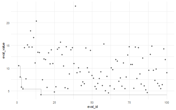
ggplot(dat, aes(x = eval_id, y = eval_value)) +
  geom_point(alpha = 0.5) +
  geom_step(aes(x = eval_id, y = min_eval), alpha = 0.3) +
  theme_minimal()