Network
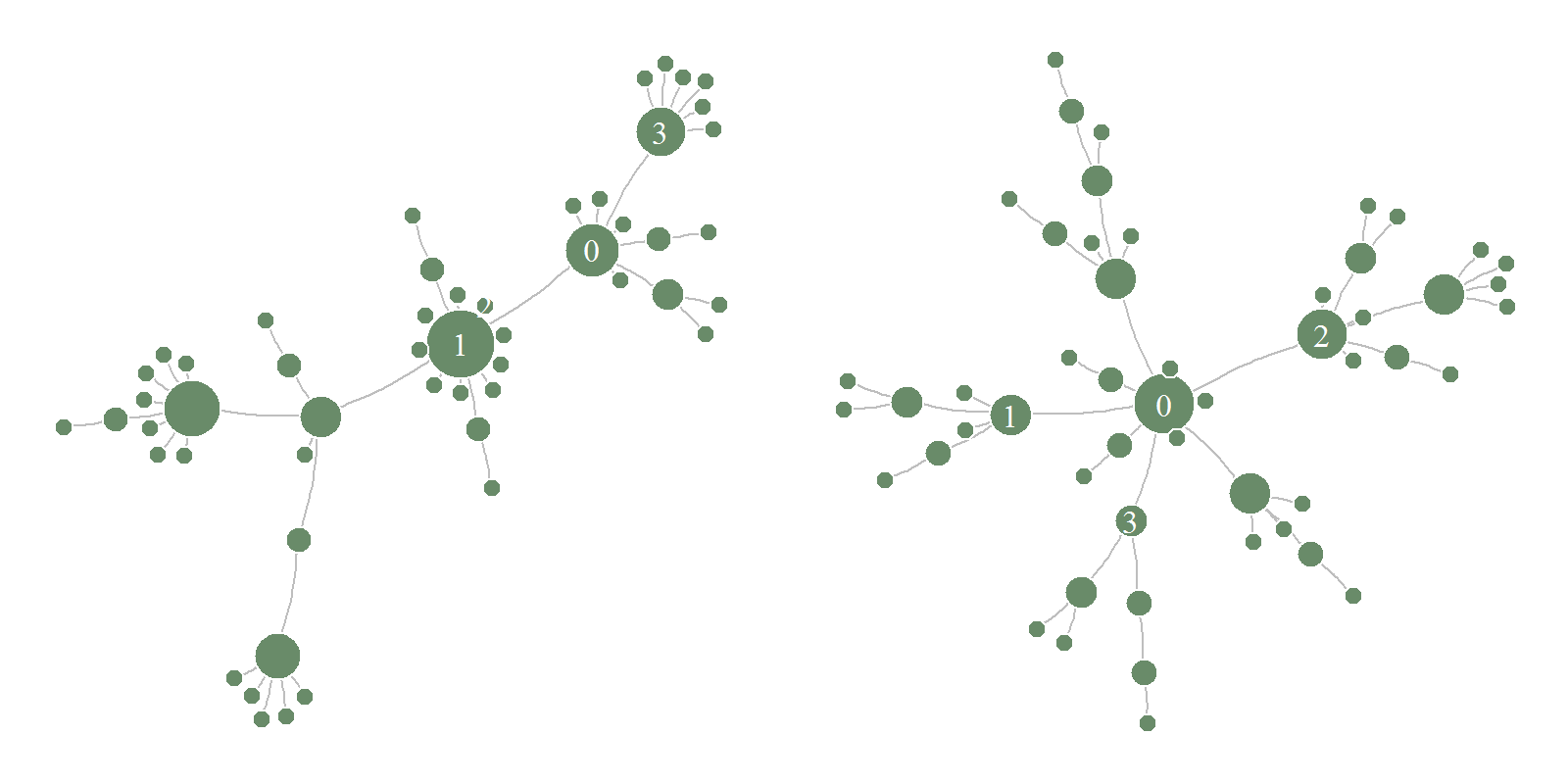
Example below shows usage of agents_after element to read the network structure from Netlogo Preferential attachment model (Wilensky, 2005).
To get data about agents use agents_after argument with a list of agents variables and type of agent (turtles and links in this example).
Element agents_before is analogous tp agents_after - it just gets the data before model runs.
experiment <- nl_experiment(
  model_file =
    file.path(nl_netlogo_path(),
              "models/Sample models/Networks/Preferential attachment.nlogo"),
  iterations = 50,
  agents_after = list(
    vertices = agent_set(
      vars = c("who", "xcor", "ycor"),
      agents = "turtles"),
    edges = agent_set(
      vars = c(e1 = "[who] of end1", e2 ="[who] of end2"),
      agents = "links")
  ),
  repetitions = 2,
  random_seed = c(42, 69)
)result <- nl_run(experiment)
#> Warning: Parameter sets not defined. Using default parametersThe data about individual agents are now stored in result$agents_after$edges and result$agents_after$vertices. To join the data with parameter sets use nl_get_result(result, type = "agents_after", sub_type = "edges")
With igraph package one can recreate the graph structure from agents’ data:
library(igraph, quietly = TRUE, warn.conflicts = FALSE)
glist <-
  lapply(
    1:experiment$run_options$repetitions,
    function(i){
      g_edges <- subset(result$agents_after$edges, run_id == i)
      g1 <- graph.data.frame(g_edges, directed = FALSE)
      V(g1)$size <- sqrt(degree(g1))*6
      V(g1)$label <-
        ifelse(as.numeric(V(g1)$name) < 4, as.numeric(V(g1)$name), NA)
      g1
    }
)par(mfrow=c(1,2), mai=c(0,0,0,0))
for(g1 in glist) {
plot.igraph(g1, margin = 0,
vertex.label.font = V(g1)$size * 0.07,
vertex.label.color = "white",
vertex.color="darkseagreen4",
edge.color = "gray",
vertex.frame.color="#ffffff",
edge.curved=.1
)
}
