Random Sampling

This example is using NetLogo Flocking model (Wilensky, 1998) to demonstrate sensitivity analysis with random sampling and scatter plots.

As in flocking example two measures of self-organization are defined:

converergence is based on variance of birds’ orientations and
mean crowding is average group size as experienced by individual.

Additionaly (because these measures are temporal):

criteria evaluation expressions are aggregating those measures over time (note the eval_criteria element).

A list of parameter values in the param_values argument would be interpreted as all combinations of parameter values. In this example parameter values are defined with nl_param_lhs function. It uses Latin Hypercube sampling to create \(n\) random parameter value sets.

Note that two values are sufficient to define a parameter value range.

Parameters with only one value (population and world_size in this example) are treated as constants.

The NetLogo Flocking model is non-deterministic (birds are oriented randomly at setup) and simulation repeats several times (10 in this example) for each parameter value set (set by repetitions argument).

With random_seed argument we gain reproducibility but it must be set with different values for every repetition (in this example it is a vector of size 10).

experiment <- nl_experiment( 
  model_file = "models/Sample Models/Biology/Flocking.nlogo",
  setup_commands = c("setup", "repeat 100 [go]"),
  iterations = 5,

  param_values = nl_param_lhs(   # create 100 parameter value sets with LHS
    n = 100,
    world_size = 50,
    population = 80,
    max_align_turn = c(0, 20),
    max_cohere_turn = c(0, 20),
    max_separate_turn = c(0, 20),
    vision = c(1, 10),
    minimum_separation = c(0, 10),
    .dummy = c(0, 1) 
  ),
  mapping = nl_default_mapping, 

  step_measures = measures(
    converged = "1 - 
      (standard-deviation [dx] of turtles + 
       standard-deviation [dy] of turtles) / 2",
    mean_crowding = 
      "mean [count flockmates + 1] of turtles"
  ),
  eval_criteria = criteria(
    c_converged = mean(step$converged),
    c_mcrowding = mean(step$mean_crowding)
  ),

  repetitions = 10,                        # repeat simulations 10 times
  random_seed = 1:10

)

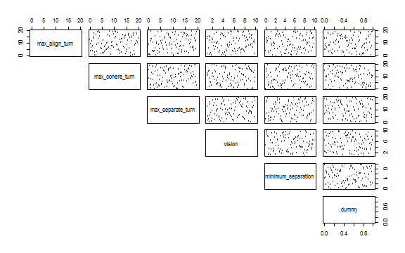
To see the experiment design with scatter plots use nl_show_params function:

nl_show_params(experiment)

Run the experiment:

result <- nl_run(experiment, parallel = TRUE)

dat <- nl_get_result(result, type = "criteria")

library(tidyr)
dat_long <- gather_(dat, key = "parameter", value = "value", 
                c("max_align_turn", "max_cohere_turn", "max_separate_turn", 
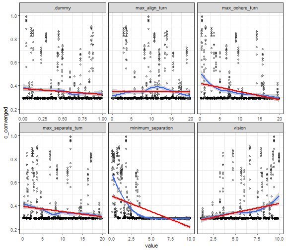
                  "vision", "minimum_separation", ".dummy"))

Convergence sensitivity:

library(ggplot2)
ggplot(dat_long, aes(x = value, y = c_converged)) +
  geom_point(alpha = 0.3) +
  stat_smooth(method = "loess") +
  stat_smooth(method = "lm", color = "red") +
  facet_wrap(~ parameter, scales = "free_x") + 
  theme_bw()

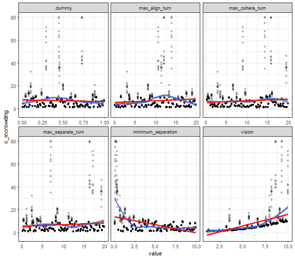
Mean crowding sensitivity:

ggplot(dat_long, aes(x = value, y = c_mcrowding)) +
  geom_point(alpha = 0.2) +
  stat_smooth(method = "loess") +
  stat_smooth(method = "lm", color = "red") +
  facet_wrap(~ parameter, scales = "free_x") + 
  theme_bw()

Random Sampling

Related